05 Electronic Bands - conocimientos.com.ve

the tight binding model

Is an approach to the calculation of electronic band structure using an approximate set of wave functions based upon superposition of wave functions for isolated atoms located at each atomic site. The method is closely related to the linear combination of atomic orbitals molecular orbital method used for molecules. Tight binding calculates the ground state electronic energy and position of bandgaps for a molecule.

Background

This approximation could be considered the analog of the LCAO (Linear Combination of Atomic Orbital) approach used in molecular physics. Like the LCAO approach, the atomic locations can be specified arbitrarily (or additional calculations can be done to find the atomic positions), so the method can be applied to non-crystalline materials. However, the most common applications are to crystalline materials where the atomic positions are located on a periodic space lattice of sites.
In this approach, interactions between different atomic sites are considered as perturbations. There exists several kinds of interactions we must consider. The crystal Hamiltonian is only approximately a sum of atomic Hamiltonians located at different sites and atomic wave functions overlap adjacent atomic sites in the crystal, and so are not accurate representations of the exact wave function. There are further explanations in the next section with some mathematical expressions.
Recently, in the research about strongly correlated material, the tight binding approach is basic approximation because highly localized electrons like 3-d transition metal electrons sometimes indicate strongly correlated behaviors. In this case, the role of electron-electron interaction must be considered using the many-body physics description.
The tight-binding model is typically used for calculations of electronic band structure and band gaps in the static regime. However, in combination with other methods such as the random phase approximation (RPA) model, the dynamic response of systems may also be studied.

Formulation

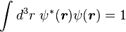
We introduce the atomic orbitals φ_m( r ), which are eigenfunctions of the Hamiltonian H_at of a single isolated atom. When the atom is placed in a crystal, this atomic wave function overlaps adjacent atomic sites, and so are not true eigenfunctions of the crystal Hamiltonian. The overlap is less when electrons are tightly bound, which is the source of the descriptor "tight-binding". Any corrections to the atomic potential ΔU required to obtain the true Hamiltonian H of the system, are assumed small:

$H (\boldsymbol{r}) = \sum_{\boldsymbol{R_n}} H_{\mathrm{at}}(\boldsymbol{r - R_n}) +\Delta U (\boldsymbol{r}) \ .$

A solution ψ(r) to the time-independent single electron Schrödinger equation is then approximated as a linear combination of atomic orbitals φ_m( r − R_n ):

$\psi(\boldsymbol{r}) = \sum_{m,\boldsymbol{R_n}} b_m ( \boldsymbol{R_n}) \ \varphi_m (\boldsymbol{r-R_n})$ ,

where m refers to the m-th atomic energy level and R_n locates an atomic site in the crystal lattice.
The translational symmetry of the crystal implies the wave function under translation can change only by a phase factor:

$\psi(\boldsymbol{r+R_{\ell}}) = e^{i\boldsymbol{k \cdot R_{\ell}}}\psi(\boldsymbol{r}) \ ,$

where k is the wave vector of the wave function. Consequently, the coefficients satisfy

$\sum_{m,\boldsymbol{R_n}} b_m ( \boldsymbol{R_n}) \ \varphi_m (\boldsymbol{r-R_n+R_{\ell}})=e^{i\boldsymbol{k \cdot R_{\ell}}}\sum_{m,\boldsymbol{R_n}} b_m ( \boldsymbol{R_n}) \ \varphi_m (\boldsymbol{r-R_n})\ .$

By substituting R_p = R_n − R_ℓ, we find

$b_m ( \boldsymbol{R_p+R_{\ell}}) = e^{i\boldsymbol{k \cdot R_{\ell}}}b_m ( \boldsymbol{R_p}) \ ,$

$b_m (\boldsymbol{R_p}) = e^{i\boldsymbol{k \cdot R_{p}}} b_m ( \boldsymbol{0}) \ .$

Normalizing the wave function to unity:

$\int d^3 r \ \psi^* (\boldsymbol{r}) \psi (\boldsymbol{r}) = 1$

$= \sum_{\boldsymbol{R_n}} b^* ( \boldsymbol{R_n})\sum_{\boldsymbol{R_{\ell}}} b ( \boldsymbol{R_{\ell}})\int d^3 r \ \varphi^* (\boldsymbol{r-R_n}) \varphi (\boldsymbol{r-R_{\ell}})$

$= b^*(0)b(0)\sum_{\boldsymbol{R_n}} e^{-i \boldsymbol{k \cdot R_n}}\sum_{\boldsymbol{R_{\ell}}} e^ {i \boldsymbol{k \cdot R_{\ell}}}\ \int d^3 r \ \varphi^* (\boldsymbol{r-R_n}) \varphi (\boldsymbol{r-R_{\ell}})$

$=N b^*(0)b(0)\sum_{\boldsymbol{R_p}} e^{-i \boldsymbol{k \cdot R_p}}\ \int d^3 r \ \varphi^* (\boldsymbol{r-R_p}) \varphi (\boldsymbol{r})\$

$=N b^*(0)b(0)\sum_{\boldsymbol{R_p}} e^{i \boldsymbol{k \cdot R_p}}\ \int d^3 r \ \varphi^* (\boldsymbol{r}) \varphi (\boldsymbol{r-R_p})\ ,$

so the normalization sets b(0) as

$b^*(0)b(0) = \frac {1} {N}\ \cdot \ \frac {1}{1 + \sum_{\boldsymbol{R_p \neq 0}} e^{-i \boldsymbol{k \cdot R_p}} \alpha (\boldsymbol{R_p})} \ ,$

where α (R_p ) are the atomic overlap integrals, which frequently are neglected resulting in^[1]

$b_n (0) \approx \frac {1} {\sqrt{N}} \ ,$

and

$\psi (\boldsymbol{r}) \approx \frac {1} {\sqrt{N}} \sum_{m,\boldsymbol{R_n}} e^{i \boldsymbol{k \cdot R_n}} \ \varphi_m (\boldsymbol{r-R_n}) \ .$

Using the tight binding form for the wave function, and assuming only the m-th atomic energy level is important for the m-th energy band, the Bloch energies $\varepsilon_m$ are of the form

$\varepsilon_m = \int d^3 r \ \psi^* (\boldsymbol{r})H(\boldsymbol{r}) \psi (\boldsymbol{r})$

$=\sum_{\boldsymbol{R_n}} b^* ( \boldsymbol{R_n})\ \int d^3 r \ \varphi^* (\boldsymbol{r-R_n})H(\boldsymbol{r}) \psi (\boldsymbol{r}) \$

$=\sum_{\boldsymbol{R_{\ell}}} \ \sum_{\boldsymbol{R_n}} b^* ( \boldsymbol{R_n})\ \int d^3 r \ \varphi^* (\boldsymbol{r-R_n})H_{\mathrm{at}}(\boldsymbol{r-R_{\ell}}) \psi (\boldsymbol{r}) \ + \sum_{\boldsymbol{R_n}} b^*( \boldsymbol{R_n})\ \int d^3 r \ \varphi^* (\boldsymbol{r-R_n})\Delta U (\boldsymbol{r}) \psi (\boldsymbol{r}) \ .$

$\approx E_m + b^*(0)\sum_{\boldsymbol{R_n}} e^{-i \boldsymbol{k \cdot R_n}}\ \int d^3 r \ \varphi^* (\boldsymbol{r-R_n})\Delta U (\boldsymbol{r}) \psi (\boldsymbol{r}) \ .$

Here terms involving the atomic Hamiltonian at sites other than where it is centered are neglected. The energy then becomes

$\varepsilon_m(\boldsymbol{k}) = E_m - N\ |b (0)|^2 \left(\beta_m + \sum_{\boldsymbol{R_n}\neq 0} \gamma_m(\boldsymbol{R_n}) e^{i \boldsymbol{k} \cdot \boldsymbol{R_n}}\right) \ ,$

$= E_m - \ \frac {\beta_m + \sum_{\boldsymbol{R_n}\neq 0} \gamma_m(\boldsymbol{R_n}) e^{i \boldsymbol{k} \cdot \boldsymbol{R_n}}}{1 + \sum_{\boldsymbol{R_n \neq 0}} e^{i \boldsymbol{k \cdot R_n}} \alpha (\boldsymbol{R_n})} \ ,$

where E_m is the energy of the m-th atomic level,

$\beta_m = -\int \varphi_m^*(\boldsymbol{r})\Delta U(\boldsymbol{r}) \varphi_m(\boldsymbol{r}) \, d^3 r \$ ,

$\gamma_m(\boldsymbol{R_n}) = -\int \varphi_m^*(\boldsymbol{r}) \Delta U(\boldsymbol{r}) \varphi_m(\boldsymbol{r - R_n}) \, d^3 r \ ,$

and

$\alpha_m(\boldsymbol{R_n}) = \int \varphi_m^*(\boldsymbol{r}) \varphi_m(\boldsymbol{r - R_n}) \, d^3 r \$ ,

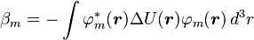
are the overlap integrals.

One-dimensional example

Here the tight binding model is illustrated for a string of atoms in a straight line with spacing a between atomic sites. Denote the translation operator

τ

, which satisfies the property:^[2]

$\tau(a)|n\rangle =|n+1\rangle$

Here, the state ket $|n\rangle$ represents a particular choice of atomic orbital (for example, an s- or p- orbital from some shell of orbitals) located at the site R_n = n a in the lattice with lattice constant a. Because the Hamiltonian

H

is invariant under the operation

τ(a)

, we have commutation relation

$[H,\ \tau{(a)}]=0$ .

This commutation relation implies the Hamiltonian operator

H

and translation operator

τ(a)

can be simultaneously diagonalized.
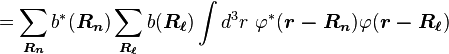
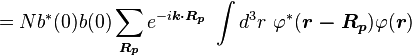
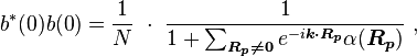
To find approximate eigenstates of the Hamiltonian, we can use a linear combination of the atomic orbitals

$|k\rangle =\frac{1}{\sqrt{N}}\sum_{n=1}^N e^{inka} |n\rangle$

where N = total number of sites and

k

is a real parameter with $-\frac{\pi}{a}\leqq k\leqq\frac{\pi}{a}$ . (This wave function is normalized to unity by the leading factor 1/√N provided overlap of atomic wave functions is ignored.) If we apply the lattice translation operator

τ(a)

to this state $|k\rangle$ , this state is found to be an eigenstate of this operator:

$\tau(a)|k\rangle=\frac{1}{\sqrt{N}}\sum_n e^{inka}|n+1\rangle=\frac{1}{\sqrt{N}}\sum_n e^{i(n-1)ka}|n\rangle = e^{ika}|k\rangle$

Assuming only nearest neighbor overlap (that is, tight binding), the only non-zero matrix elements of the Hamiltonian can be expressed as

$\langle n\pm 1|H|n\rangle=-\Delta \ ;$ $\langle n|H|n\rangle=E_0 \ .$

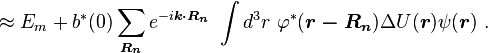
The energy E₀ is approximately the atomic energy level corresponding to the chosen atomic orbital if H at site R_n = n a is approximately H_at at that site. We can derive the energy of the state $|k\rangle$ using the above equation:

$H|k\rangle=\frac{1}{\sqrt{N}}\sum_n e^{inka} H |n\rangle$

$\langle k| H|k\rangle =\frac{1}{N}\sum_{n,\ m} e^{i(n-m)ka} \langle m|H|n\rangle$ $=\frac{1}{N}\sum_n \langle n|H|n\rangle+\frac{1}{N}\sum_n \langle n-1|H|n\rangle e^{+ika}+\frac{1}{N}\sum_n\langle n+1|H|n\rangle e^{-ika}$ $= E_0 -2\Delta\,\cos(ka)\ ,$

where, for example,

$\frac{1}{N}\sum_n \langle n|H|n\rangle = E_0 \frac{1}{N}\sum_n 1 = E_0 \ ,$

and

$\frac{1}{N}\sum_n \langle n-1|H|n\rangle e^{+ika}=-\Delta e^{ika}\frac{1}{N}\sum_n 1 = -\Delta e^{ika} \ .$

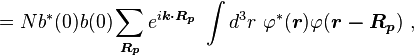
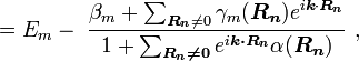
Thus the energy of this state $|k\rangle$ can be represented in the familiar form of the energy dispersion:

$E(k)=E_0-2\Delta\,\cos(ka)$ .

This example is readily extended to three dimensions, for example, to a body-centered cubic or face-centered cubic lattice by introducing the nearest neighbor vector locations in place of simply n a.^[3] Likewise, the method can be extended to multiple bands using multiple different atomic orbitals at each site. The general formulation above shows how these extensions can be accomplished.

Connection to Wannier functions

Bloch wave functions describe the electronic states in a periodic crystal lattice. Bloch functions can be represented as a Fourier series ^[4]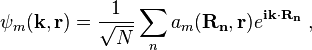

$\psi_m\mathbf{(k,r)}=\frac{1}{\sqrt{N}}\sum_{n}{a_m\mathbf{(R_n,r)}} e^{\mathbf{ik\cdot R_n}}\ ,$

where R_n denotes an atomic site in a periodic crystal lattice, k is the wave vector of the Bloch wave, r is the electron position, m is the band index, and the sum is over all N atomic sites. The Bloch wave is an exact eigensolution for the wave function of an electron in a periodic crystal potential corresponding to an energy E_m (k), and is spread over the entire crystal volume.
Using the Fourier transform analysis, a spatially localized wave function for the m-th energy band can be derived from this Bloch wave:

$a_m\mathbf{(R_n,r)}=\frac{1}{\sqrt{N}}\sum_{\mathbf{k}}{e^{\mathbf{-ik\cdot R_n}}\psi_m\mathbf{(k,r)}}=\frac{1}{\sqrt{N}}\sum_{\mathbf{k}}{e^{\mathbf{ik\cdot (r-R_n)}}u_m\mathbf{(k,r)}}.$

These real space wave functions ${a_m\mathbf{(R_n,r)}}$ are called Wannier functions, and are fairly closely localized to the atomic site R_n. Of course, if we have exact Wannier functions, the exact Bloch functions can be derived using the inverse Fourier transform.
However it is not easy to calculate directly either Bloch functions or Wannier functions. An approximate approach is necessary in the calculation of electronic structures of solids. If we consider the extreme case of isolated atoms, the Wannier function would become an isolated atomic orbital. That limit suggests the choice of an atomic wave function as an approximate form for the Wannier function, the so-called tight binding approximation.

Second quantization

Modern explanations of electronic structure like t-J model and Hubbard model are based on tight binding model.^[5] If we introduce second quantization formalism, it is clear to understand the concept of tight binding model.
Using the atomic orbital as a basis state, we can establish the second quantization Hamiltonian operator in tight binding model.

$H = -t \sum_{\langle i,j \rangle,\sigma}( c^{\dagger}_{i,\sigma} c^{}_{j,\sigma}+ h.c.)$ ,

$c^\dagger_{i\sigma} , c_{j\sigma}$ - creation and annihilation operators

$\displaystyle\sigma$ - spin polarization

$\displaystyle t$ - hopping integral

$\displaystyle \langle i,j \rangle$ -nearest neighbor index

Here, hopping integral $\displaystyle t$ corresponds to the transfer integral $\displaystyle\gamma$ in tight binding model. Considering extreme cases of $t\rightarrow 0$ , it is impossible for electron to hop into neighboring sites. This case is the isolated atomic system. If the hopping term is turned on ( $\displaystyle t>0$ ) electrons can stay in both sites lowering their kinetic energy.
In the strongly correlated electron system, it is necessary to consider the electron-electron interaction. This term can be written in

$\displaystyle H_{ee}=\frac{1}{2}\sum_{n,m,\sigma}\langle n_1 m_1, n_2 m_2|\frac{e^2}{|r_1-r_2|}|n_3 m_3, n_4 m_4\rangle c^\dagger_{n_1 m_1 \sigma_1}c^\dagger_{n_2 m_2 \sigma_2}c_{n_4 m_4 \sigma_2} c_{n_3 m_3 \sigma_1}$

This interaction Hamiltonian includes direct Coulomb interaction energy and exchange interaction energy between electrons. There are several novel physics induced from this electron-electron interaction energy, such as metal-insulator transitions (MIT), high-temperature superconductivity, and several quantum phase transitions.

Agustin Egui
EES

Navega con el navegador más seguro de todos. ¡Descárgatelo ya!

05 Electronic Bands - conocimientos.com.ve

lunes, 15 de febrero de 2010

Background

Formulation

One-dimensional example

Connection to Wannier functions

Second quantization

No hay comentarios:

Publicar un comentario